Understanding Normal Random Number Simulation

This document explores the simulation of normal random numbers in Python through the Box-Muller method.

"Inverse Sampling can be applied to various probability distributions, but it is crucial that the cumulative distribution function can be expressed in a closed-form and is invertible."

For normal random variables, the probability density function is represented as follows:

The error function, denoted as erf(x), plays a significant role in this context. We can also express this function as:

Next, we would typically seek an inverse function for ?(z). However, since erf(x) lacks a closed-form inverse, utilizing this method for sampling normally distributed numbers becomes problematic. So, what alternatives do we have?

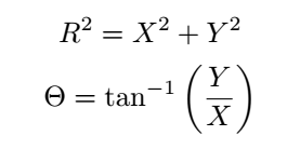
According to the Box-Muller method, if A and B are two independent uniformly distributed random numbers (e.g., A~Uniform(0,1), B~Uniform(0,1)), you can generate normally distributed random numbers X and Y as follows:

While the theoretical underpinnings are intricate and beyond the scope of this discussion, let's see how this works in practice. The following Python script demonstrates this process:

# Generating Normal Random Numbers

# Author: Oscar A. Nieves

# Last updated: July 01, 2021

import matplotlib.pyplot as plt

import numpy as np

plt.close('all')

np.random.seed(0) # Setting the random seed

# Inputs

mu = 0.5

sigma = 0.75

samples = 100000

# Random samples (Uniformly distributed)

A = np.random.rand(samples, 1)

B = np.random.rand(samples, 1)

# Normal random numbers N(mu, sigma^2)

X = np.sqrt(-2 * np.log(A)) * np.cos(2 * np.pi * B)

Y = np.sqrt(-2 * np.log(A)) * np.sin(2 * np.pi * B)

# Compute statistics

EX = round(np.mean(X), 2)

VarX = round(np.var(X), 2)

EY = round(np.mean(Y), 2)

VarY = round(np.var(Y), 2)

# Plot histograms

bins = 50

plt.subplot(1, 2, 1)

plt.hist(X, bins)

plt.xlabel('X ~ N(mu = ' + str(EX) + ', sigma^2 = ' + str(VarX) + ')', fontsize=16)

plt.ylabel('frequency', fontsize=16)

plt.subplot(1, 2, 2)

plt.hist(Y, bins)

plt.xlabel('Y ~ N(mu = ' + str(EY) + ', sigma^2 = ' + str(VarY) + ')', fontsize=16)

plt.ylabel('frequency', fontsize=16)

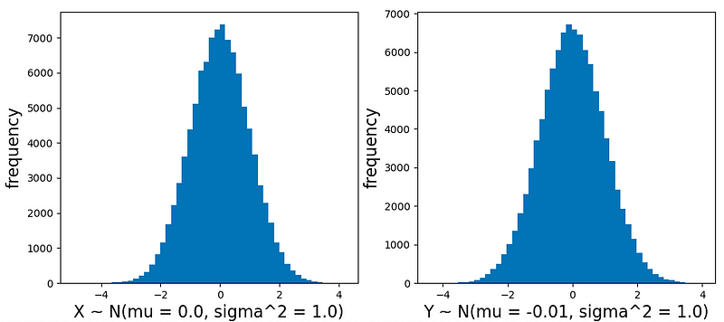
Upon executing this code, the resulting plots are:

Here, we observe that both X and Y exhibit a mean of 0 and a variance of 1, indicating that they conform to a standard normal distribution, as anticipated by the method.

Now, the pressing question is: how can we generate X and Y to have specific means and variances other than 0 and 1? This can be achieved by leveraging the properties of normal random variables. If Z is normally distributed with mean μ and variance σ², we can express this as:

Consequently, for our scenario, we can express X and Y as:

By modifying our Python code accordingly:

# Normal random numbers N(mu, sigma^2)

X = mu + sigma * np.sqrt(-2 * np.log(A)) * np.cos(2 * np.pi * B)

Y = mu + sigma * np.sqrt(-2 * np.log(A)) * np.sin(2 * np.pi * B)

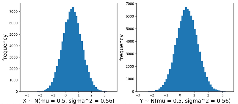
we can now achieve:

Both variables now have a mean of μ = 0.5 and a variance of 0.56 (corresponding to our σ = 0.75).

Now, you are equipped with the knowledge to sample normally distributed random numbers using only uniformly distributed random numbers. Enjoy your exploration!

Chapter 2: Additional Resources

To deepen your understanding, refer to the following videos:

This video explains how to generate random numbers in Python using NumPy, including both floats and integers.

Learn how to generate random numbers in Python, with practical examples and clear explanations.